Basic Example

In this notebook, we will see how to use Polire for spatial interpolation.

import numpy as np
import xarray as xr
import pandas as pd
import matplotlib.pyplot as plt

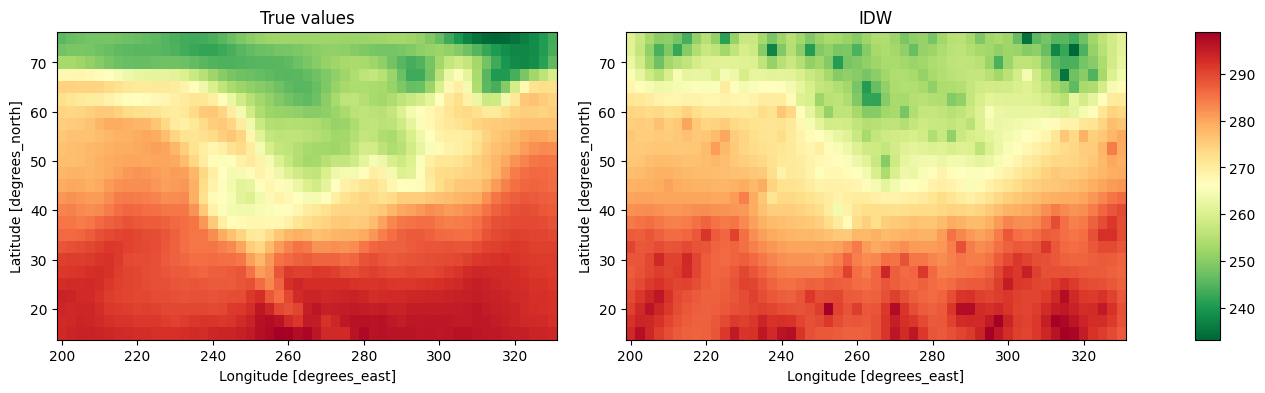
import polire
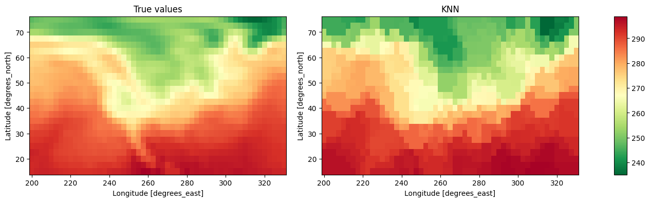
from sklearn.neighbors import KNeighborsRegressor
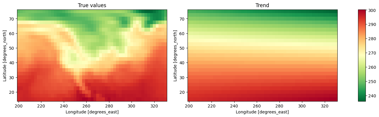
from sklearn.linear_model import LinearRegression
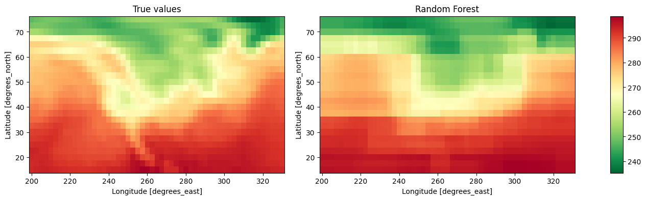
from sklearn.ensemble import RandomForestRegressor

from sklearn.metrics import (
    mean_squared_error,
    mean_absolute_error,
    mean_absolute_percentage_error,
    r2_score,
)

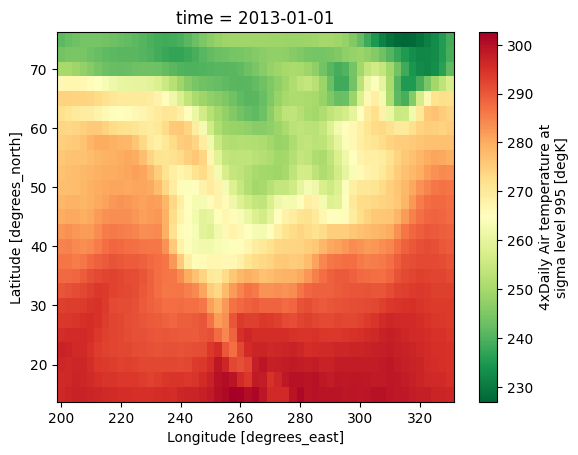
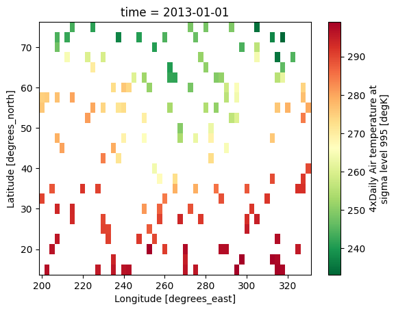
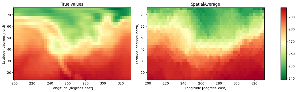
# set default cmap
plt.rcParams["image.cmap"] = "RdYlGn_r"
xr.set_options(cmap_sequential="RdYlGn_r")

<xarray.core.options.set_options at 0x7fc3b0198c40>

Load the data

ds = xr.tutorial.open_dataset("air_temperature")
ds

<xarray.Dataset>
Dimensions:  (lat: 25, time: 2920, lon: 53)
Coordinates:
  * lat      (lat) float32 75.0 72.5 70.0 67.5 65.0 ... 25.0 22.5 20.0 17.5 15.0
  * lon      (lon) float32 200.0 202.5 205.0 207.5 ... 322.5 325.0 327.5 330.0
  * time     (time) datetime64[ns] 2013-01-01 ... 2014-12-31T18:00:00
Data variables:
    air      (time, lat, lon) float32 ...
Attributes:
    Conventions:  COARDS
    title:        4x daily NMC reanalysis (1948)
    description:  Data is from NMC initialized reanalysis\n(4x/day).  These a...
    platform:     Model
    references:   http://www.esrl.noaa.gov/psd/data/gridded/data.ncep.reanaly...

xarray.Dataset

• Dimensions:
  • lat: 25
  • time: 2920
  • lon: 53
• Coordinates: (3)
  • lat
    (lat)
    float32
    75.0 72.5 70.0 ... 20.0 17.5 15.0

    standard_name :

    latitude

    long_name :

    Latitude

    units :

    degrees_north

    axis :

    Y

    array([75. , 72.5, 70. , 67.5, 65. , 62.5, 60. , 57.5, 55. , 52.5, 50. , 47.5,
           45. , 42.5, 40. , 37.5, 35. , 32.5, 30. , 27.5, 25. , 22.5, 20. , 17.5,
           15. ], dtype=float32)

  • lon
    (lon)
    float32
    200.0 202.5 205.0 ... 327.5 330.0

    standard_name :

    longitude

    long_name :

    Longitude

    units :

    degrees_east

    axis :

    X

    array([200. , 202.5, 205. , 207.5, 210. , 212.5, 215. , 217.5, 220. , 222.5,
           225. , 227.5, 230. , 232.5, 235. , 237.5, 240. , 242.5, 245. , 247.5,
           250. , 252.5, 255. , 257.5, 260. , 262.5, 265. , 267.5, 270. , 272.5,
           275. , 277.5, 280. , 282.5, 285. , 287.5, 290. , 292.5, 295. , 297.5,
           300. , 302.5, 305. , 307.5, 310. , 312.5, 315. , 317.5, 320. , 322.5,
           325. , 327.5, 330. ], dtype=float32)

  • time
    (time)
    datetime64[ns]
    2013-01-01 ... 2014-12-31T18:00:00

    standard_name :

    time

    long_name :

    Time

    array(['2013-01-01T00:00:00.000000000', '2013-01-01T06:00:00.000000000',
           '2013-01-01T12:00:00.000000000', ..., '2014-12-31T06:00:00.000000000',
           '2014-12-31T12:00:00.000000000', '2014-12-31T18:00:00.000000000'],
          dtype='datetime64[ns]')

• Data variables: (1)
  • air
    (time, lat, lon)
    float32
    ...

    long_name :

    4xDaily Air temperature at sigma level 995

    units :

    degK

    precision :

    2

    GRIB_id :

    11

    GRIB_name :

    TMP

    var_desc :

    Air temperature

    dataset :

    NMC Reanalysis

    level_desc :

    Surface

    statistic :

    Individual Obs

    parent_stat :

    Other

    actual_range :

    [185.16 322.1 ]

    [3869000 values with dtype=float32]

• Indexes: (3)
  • lat
    PandasIndex

    PandasIndex(Index([75.0, 72.5, 70.0, 67.5, 65.0, 62.5, 60.0, 57.5, 55.0, 52.5, 50.0, 47.5,
           45.0, 42.5, 40.0, 37.5, 35.0, 32.5, 30.0, 27.5, 25.0, 22.5, 20.0, 17.5,
           15.0],
          dtype='float32', name='lat'))

  • lon
    PandasIndex

    PandasIndex(Index([200.0, 202.5, 205.0, 207.5, 210.0, 212.5, 215.0, 217.5, 220.0, 222.5,
           225.0, 227.5, 230.0, 232.5, 235.0, 237.5, 240.0, 242.5, 245.0, 247.5,
           250.0, 252.5, 255.0, 257.5, 260.0, 262.5, 265.0, 267.5, 270.0, 272.5,
           275.0, 277.5, 280.0, 282.5, 285.0, 287.5, 290.0, 292.5, 295.0, 297.5,
           300.0, 302.5, 305.0, 307.5, 310.0, 312.5, 315.0, 317.5, 320.0, 322.5,
           325.0, 327.5, 330.0],
          dtype='float32', name='lon'))

  • time
    PandasIndex

    PandasIndex(DatetimeIndex(['2013-01-01 00:00:00', '2013-01-01 06:00:00',
                   '2013-01-01 12:00:00', '2013-01-01 18:00:00',
                   '2013-01-02 00:00:00', '2013-01-02 06:00:00',
                   '2013-01-02 12:00:00', '2013-01-02 18:00:00',
                   '2013-01-03 00:00:00', '2013-01-03 06:00:00',
                   ...
                   '2014-12-29 12:00:00', '2014-12-29 18:00:00',
                   '2014-12-30 00:00:00', '2014-12-30 06:00:00',
                   '2014-12-30 12:00:00', '2014-12-30 18:00:00',
                   '2014-12-31 00:00:00', '2014-12-31 06:00:00',
                   '2014-12-31 12:00:00', '2014-12-31 18:00:00'],
                  dtype='datetime64[ns]', name='time', length=2920, freq=None))

• Attributes: (5)

  Conventions :

  COARDS

  title :

  4x daily NMC reanalysis (1948)

  description :

  Data is from NMC initialized reanalysis (4x/day). These are the 0.9950 sigma level values.

  platform :

  Model

  references :

  http://www.esrl.noaa.gov/psd/data/gridded/data.ncep.reanalysis.html

Let’s visualize the spatial data from a time-stamp.

ds_spatial = ds.isel(time=0)
ds_spatial["air"].plot()
plt.show()

Let’s assume that only 10% of the data is available and try to interpolate the rest of the data.

ds_spatial_train = ds_spatial.copy()

np.random.seed(42)
ds_spatial_train["air"].values = np.where(
    np.random.rand(*ds_spatial_train["air"].shape) > 0.1,
    np.nan,
    ds_spatial_train["air"].values,
)


ds_spatial_train["air"].plot()
plt.show()

Prepare the data

train_df = ds_spatial_train["air"].to_dataframe().reset_index()
train_df = train_df.dropna()

X_train = train_df[["lat", "lon"]].values
y_train = train_df["air"].values

test_df = ds_spatial["air"].to_dataframe().reset_index()
X_test = test_df[["lat", "lon"]].values
y_test = test_df["air"].values

print(X_train.shape, y_train.shape, X_test.shape, y_test.shape)

(146, 2) (146,) (1325, 2) (1325,)

Useful plotting function

def plot_predictions(y_pred, model_name):
    fig, axes = plt.subplots(
        1, 3, figsize=(15, 4), gridspec_kw={"width_ratios": [1, 1, 0.05]}
    )

    ax = axes[0]
    ds_spatial["air"].plot(ax=ax, add_colorbar=False)
    ax.set_title("True values")

    ax = axes[1]
    ds_spatial_pred = ds_spatial_train.copy()
    ds_spatial_pred["air"].values = y_pred
    mappable = ds_spatial_pred["air"].plot(ax=ax, add_colorbar=False)
    ax.set_title(f"{model_name}")

    ax = axes[2]
    fig.colorbar(mappable, cax=ax)

Models

IDW

idw = polire.IDW(exponent=2)
idw.fit(X_train, y_train)
idw_pred = idw.predict(X_test).reshape(ds_spatial["air"].shape)

plot_predictions(idw_pred, "IDW")

/home/patel_zeel/polire/polire/idw/idw.py:82: RuntimeWarning: divide by zero encountered in divide
  weights = 1 / np.power(dist, self.exponent)
/home/patel_zeel/polire/polire/idw/idw.py:83: RuntimeWarning: invalid value encountered in divide
  result = (weights * self.y[:, None]).sum(axis=0) / weights.sum(axis=0)

Kriging

kriging = polire.Kriging(variogram_model="spherical")
kriging.fit(X_train, y_train)
kriging_pred = kriging.predict(X_test).reshape(ds_spatial["air"].shape)

plot_predictions(kriging_pred, "Kriging")

Spline

spline = polire.Spline()
spline.fit(X_train, y_train)
spline_pred = spline.predict(X_test).reshape(ds_spatial["air"].shape)

plot_predictions(spline_pred, "Spline")

/home/patel_zeel/miniconda3/envs/polire/lib/python3.10/site-packages/scipy/interpolate/_fitpack_impl.py:593: RuntimeWarning: The required storage space exceeds the available storage space.
Probable causes: nxest or nyest too small or s is too small. (fp>s)
    kx,ky=3,3 nx,ny=11,11 m=146 fp=1143.783495 s=128.911993
  warnings.warn(RuntimeWarning(_iermess2[ierm][0] + _mess))

Trend

trend = polire.Trend(order=2)
trend.fit(X_train, y_train)
trend_pred = trend.predict(X_test).reshape(ds_spatial["air"].shape)

plot_predictions(trend_pred, "Trend")

SpatialAverage

spatial_average = polire.SpatialAverage(radius=15)
spatial_average.fit(X_train, y_train)
spatial_average_pred = spatial_average.predict(X_test).reshape(ds_spatial["air"].shape)

plot_predictions(spatial_average_pred, "SpatialAverage")

LinearRegression

lr = polire.CustomInterpolator(LinearRegression())
lr.fit(X_train, y_train)
lr_pred = lr.predict(X_test).reshape(ds_spatial["air"].shape)

plot_predictions(lr_pred, "Linear Regression")

NearestNeighbors

K = 3
knn = polire.CustomInterpolator(KNeighborsRegressor(n_neighbors=K))
knn.fit(X_train, y_train)
knn_pred = knn.predict(X_test).reshape(ds_spatial["air"].shape)

plot_predictions(knn_pred, "KNN")

Random Forest

rf = polire.CustomInterpolator(RandomForestRegressor(random_state=42))
rf.fit(X_train, y_train)
rf_pred = rf.predict(X_test).reshape(ds_spatial["air"].shape)

plot_predictions(rf_pred, "Random Forest")

Checking performance

models = {
    "Inverse Distance Weighting": idw_pred,
    "Kriging (spherical)": kriging_pred,
    "Spline": spline_pred,
    "Trend": trend_pred,
    "Linear Regression": lr_pred,
    f"{K}-Nearest Neighbors": knn_pred,
    "Random Forest": rf_pred,
    "Spatial Average": spatial_average_pred,
}

result = pd.DataFrame(columns=["RMSE", "MAE", "MAPE", "Neg R2"], index=models.keys())

for model_name, y_pred in models.items():
    result.loc[model_name, "RMSE"] = mean_squared_error(
        y_test.ravel(), y_pred.ravel(), squared=False
    )
    result.loc[model_name, "MAE"] = mean_absolute_error(y_test.ravel(), y_pred.ravel())
    result.loc[model_name, "MAPE"] = mean_absolute_percentage_error(
        y_test.ravel(), y_pred.ravel()
    )
    result.loc[model_name, "Neg R2"] = -r2_score(y_test.ravel(), y_pred.ravel())

result.sort_values("RMSE").style.highlight_min(axis=0, color="green").format("{:.2f}")

	RMSE	MAE	MAPE	Neg R2
Kriging (spherical)	3.10	1.95	0.01	-0.97
Random Forest	3.96	2.74	0.01	-0.96
Spline	4.43	2.85	0.01	-0.95
3-Nearest Neighbors	4.60	3.19	0.01	-0.94
Spatial Average	6.04	4.32	0.02	-0.90
Inverse Distance Weighting	6.54	5.04	0.02	-0.88
Trend	8.02	6.30	0.02	-0.82
Linear Regression	8.46	6.98	0.03	-0.80